Machine Learning Foundations A Case Study Approach Week 2

Regression: Predicting House Price

One of the most widely used statistical tools.

The idea is really simple. Using some sets of features, model how the observations associated with these features change, as the values of the features change. In this case, house values.

A house have some set of features:

• Size of the house
• Number of bedrooms
• Number of bathrooms
• Etc.

The observation is what’s the value of the house, or the house sales price.

But regression go much beyond doing prediction tasks. It can also used for classification, as well as analyze the importance of the features themselves.

Predicting House Price

• Problem arise when predicting the value of a house

How Much The House Worth?

• Unsure how much to list the house for
• Unsure what value the house has
• How to estimate the value of the house

Check Recent Neighborhood Sales

• Look at the recent sales that occurred in the neighborhood (locally at the neighboring regions)
  • How much are the other houses sold for
  • What do these houses look like
• Record recent sales
  • What was the sales price
  • What was the size of the house sold

Plot Recent House Sales

• X-Axis: size of the house measured in square feet (sq. ft.)
• Y-Axis: sales price of the house in dollar ($)
• Point: represent some individual house sale

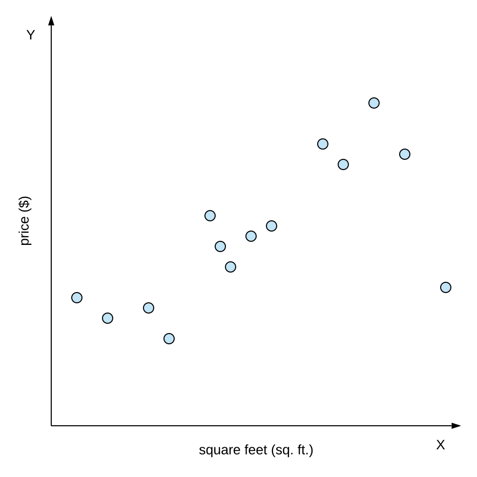
Terminology

• X: feature, covariate, or predictor (independent variable)
• Y: observation or response (dependent variable)

Predict House By Similar House

How to use these observations to estimate house value?

• Take a look how big is the house
• Look for other sales of houses of that size

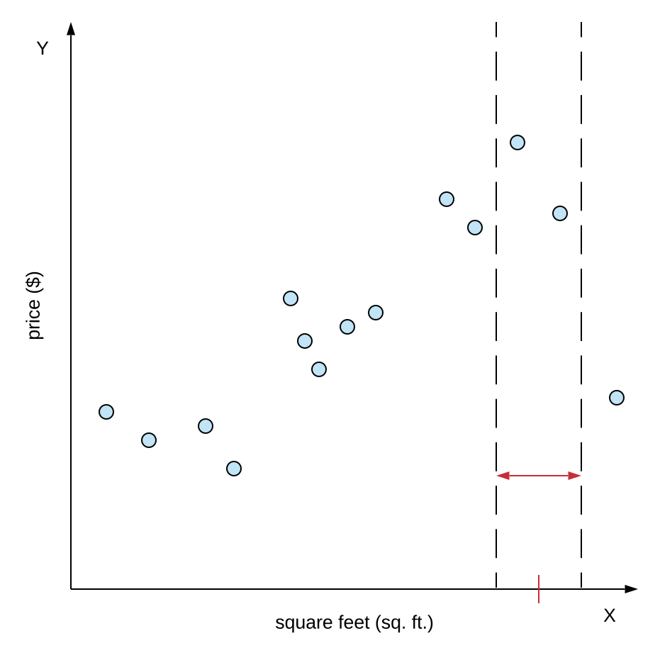
Though most likely there are going to be exactly zero house sales of the exact same square footage. Need to be a bit more flexible and look at some neighborhood (not geographic neighborhood) of range around the actual square footage.

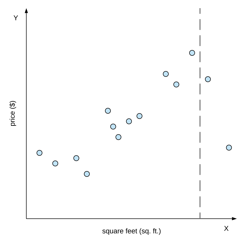
But even this approach only have two house sales to base estimate. (throwing away many other observations)

• Look at average price in range
• Still only 2 house
• Throwing out information from all other sales

Linear Regression

Think about modeling the relationship between the square footage of the house and the house sales price.

Use Linear Regression Model

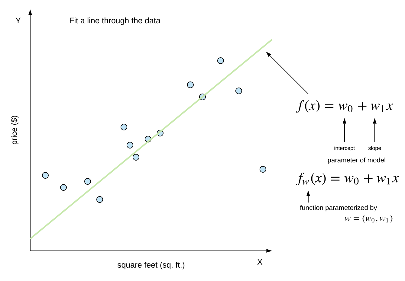
Leverage all the observations collected, understand the relationship between the square foot of the house and the house sales price. The simplest model, is just fitting a line through the data.

• Define by an intercept $w$₀ and a slope of $w$₁
• Often $w$₁ the weight on the feature $X$ or it’s called the regression coefficient
• As $X$, the square footage is varied, how much of an impact does it have on changes in the observed house sales price

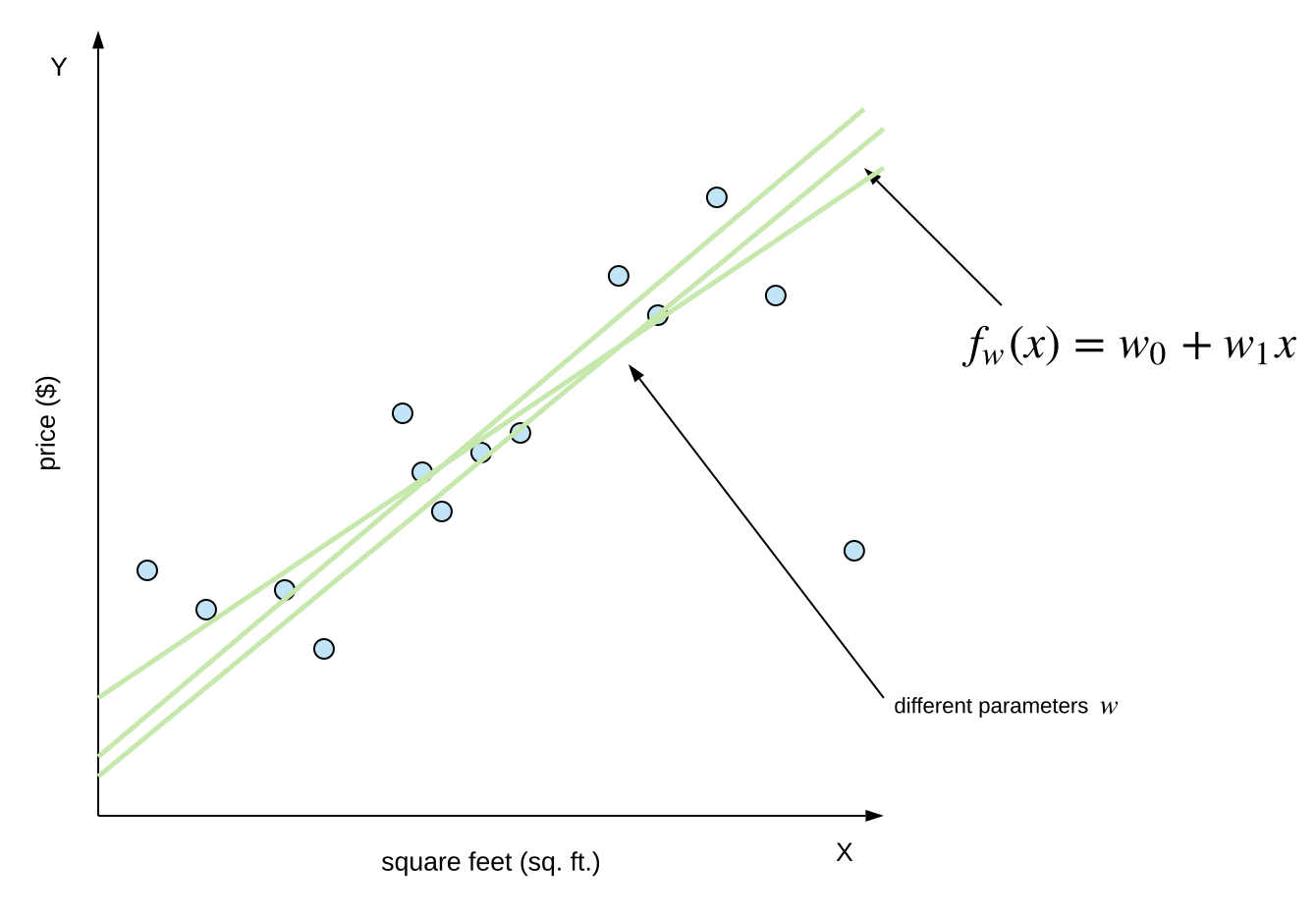
The intercept and slope are the parameters of the model. To be very explicit, the linear function with the subscript $w$ indicates the function is specified by parameters.

The $f$_w = w₀ + w₁x function parameterized by $w\; =\; (w$₀, w₁)

Which Line?

Which line is the right line or a good line to ue for a given data set? Each one is given by a different set of parameters $w$. But which $w$ to choose for the model?

Cost Using Given Line

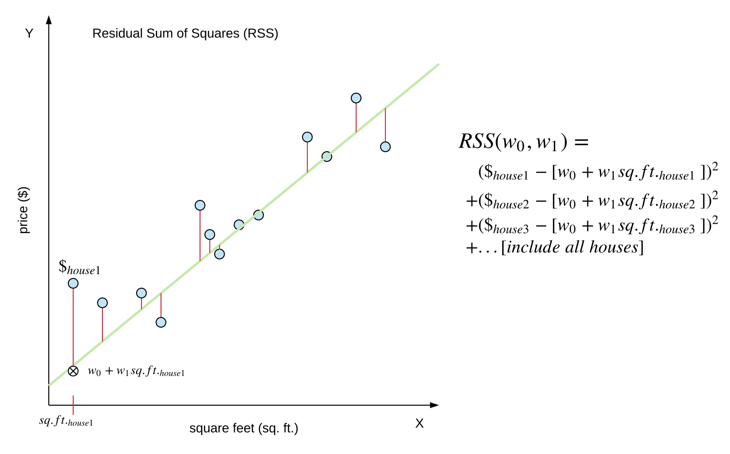
One very common cost associated with a specific fit to the data is something called the Residual Sum of Squares (RSS).

• Take the fitted line and look at each of the observations
• Look at how far is that observation from what the model would predict (point on the line)
• Look at all the distance, and look at the square of these distances
  • Called the residual, which is the difference of the prediction to the actual observation
• Look at the square and sum over them

More explicit equation

• Variable $\$$_house1 is the observed house sales price for the first house
• Variable $sq.ft.$_house1 is where the $\$$_house1 point intercept with the x-axis
• Variable $w$₀ + w₁ sq.ft._house1 is the predicted house sales price for the first house
• The difference between the observed house price versus predicted (model) for a given house square foot is $\$$_house1 - [w₀ + w₁sq.ft._house1]
• Squaring the result, and summing over all the different houses in the data set

Find Best Line

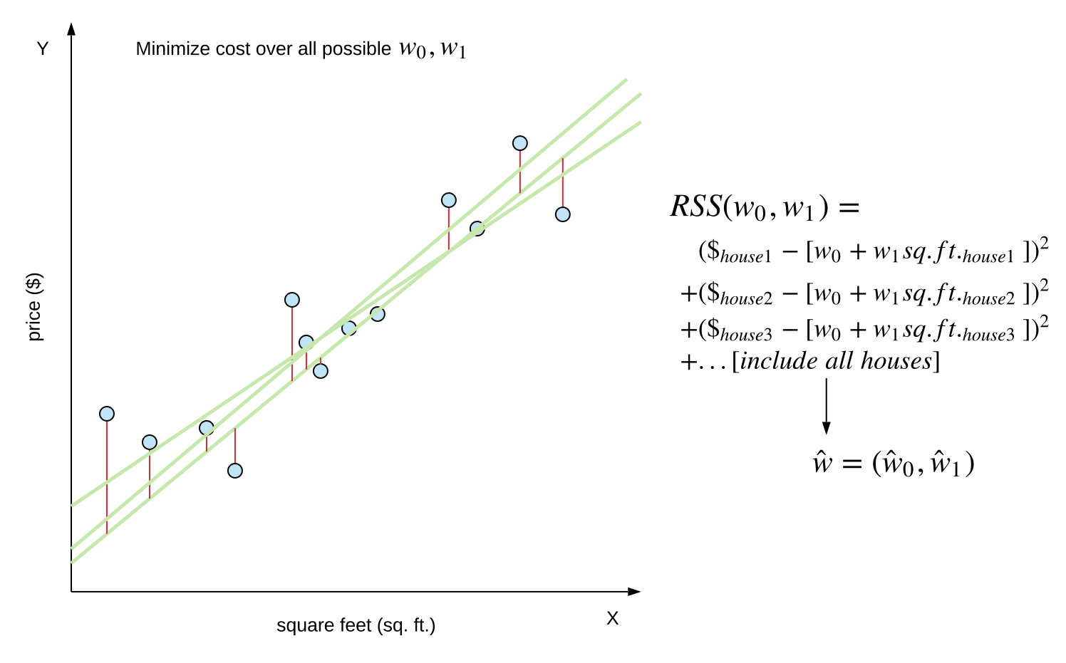
Trying to find the best line according to the metric define, the residual sum of squares.

• Search all possible $w$₀, w₁
• Search all possible lines
• Choose the one that minimize the residual sum of squares
• Denote the resulting $w$ as $ŵ$ ($w\; (hat)$)
  • It is the set of $ŵ$₀ and $ŵ$₁, which is the intercept and the slope
  • Variable $ŵ$₀ represent the set of all $w$₀
  • Variable $ŵ$₁ represent the set of all $w$₁

There exists really new and efficient algorithms for computing $ŵ$ (search over all possible $w$)

Predict House Price

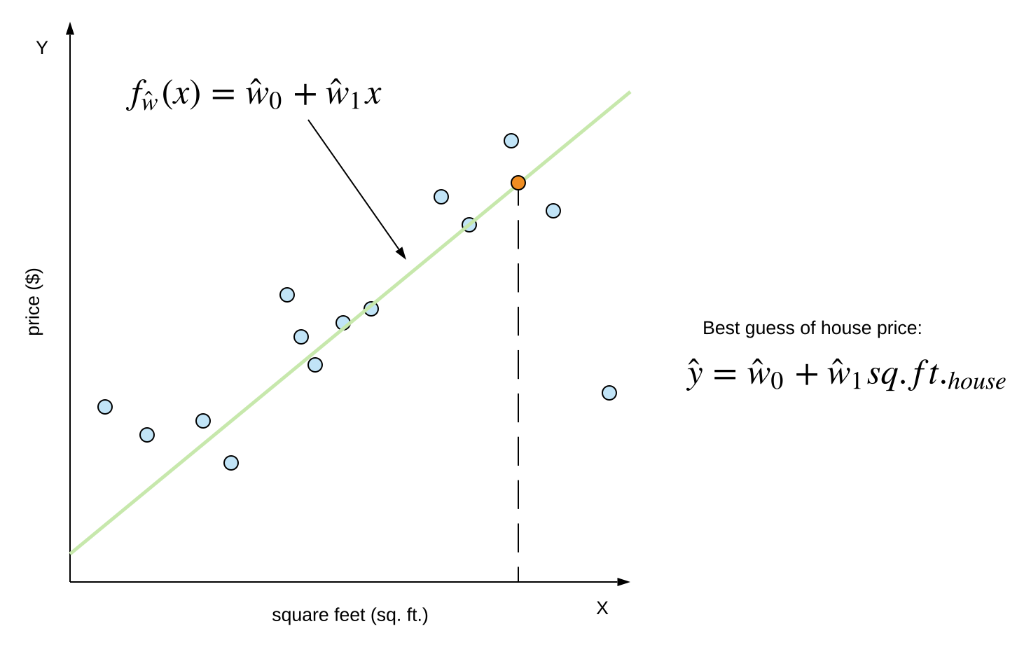
How to take the estimated model parameters and use them to predict the value of the house.

• Plotted line associated with estimate $ŵ$₀ and $ŵ$₁
• Best guess of the house price is simply what the line predicts
• Computer the value for this square footage of the house, which is $ŷ\; =\; ŵ$₀ + ŵ₁ sq.ft._house

Add Higher Order Effect

Up to this point, only considered fitting the data with a line. Is this a good choice?

Fit Data With Line?

The analysis seem to be pretty truthful.

• Fitted line
• Minimize the residual sum of squares
• Make prediction for the house value
• Leveraged all the observations recorded of all the recent house sales

Not sure this is a linear trend.

What About Quadratic Function?

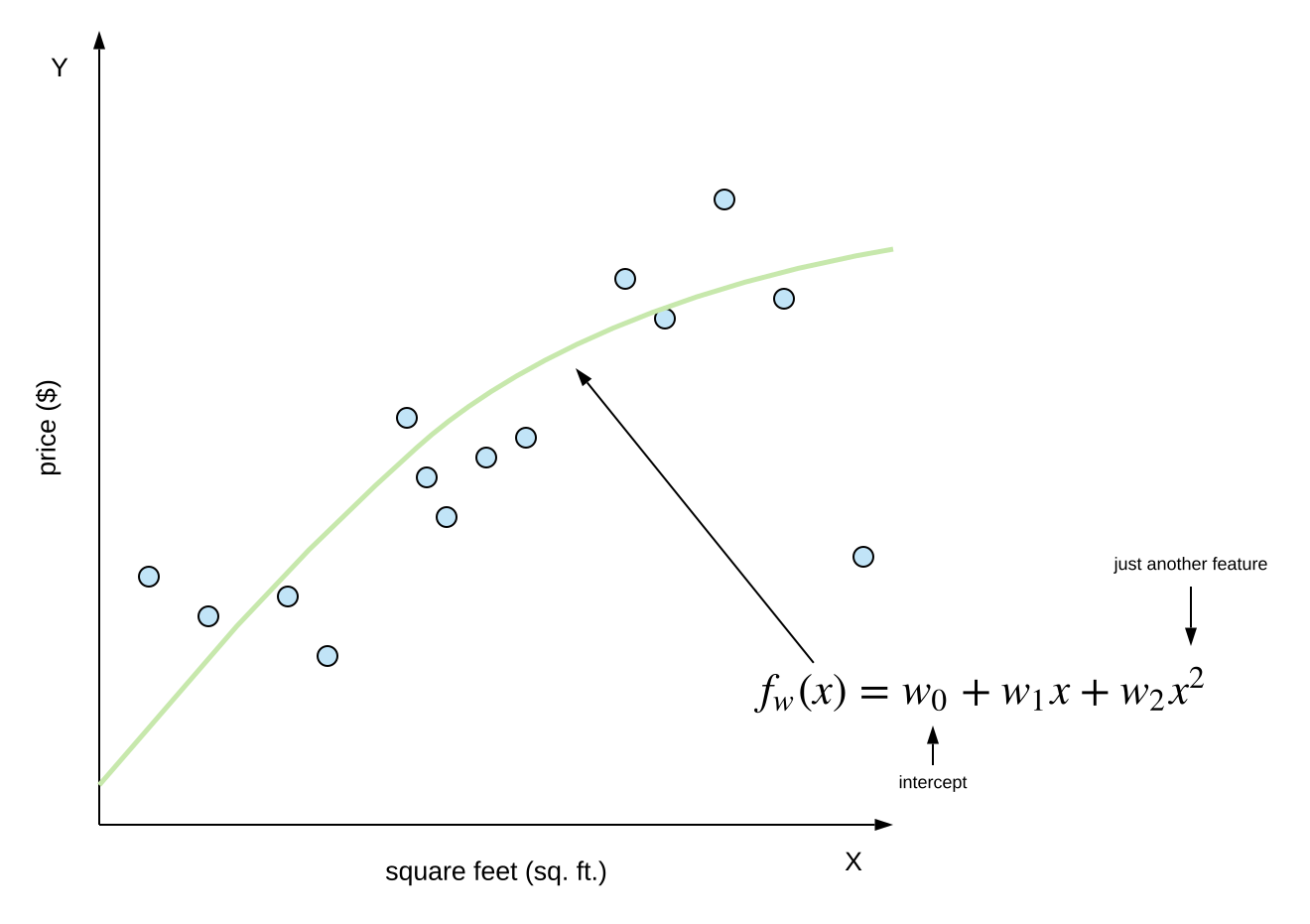
It might be quadratic. Try quadratic fit? Looking at the new plot, it actually looks pretty good. Need to figure out which is the best quadratic fit to this data, with minimizing the residual sum of squares.

Looking at the quadratic function $f$_w(x) = w₀ + w₁x + w₂x², now have 3 parameters here.

• Variable $w$₀ represent the intercept, where the curve is on the y-axis
• Variable $w$₁x represent an extra term
• Variable $w$₂x² represent the quadratic component

Despite the shape, order, and or degree of the function, it is actually still called linear regression. The variable $x2$ is just another feature. The $w$ always appear just as $w$, not $w2$ or other function of $w$.

There are currently three parameters. When minimizing residual sum of squares, need to search over the space of the three different things. It have to minimize over the combination of best $w$₀, $w$₁, and $w$₂, as well as finding the quadratic fit that minimizes the residual sum of squares.

Even Higher Order Polynomial

Try 13th order polynomial?

Believe This Fit?

• It make sense, but…
• It minimized the residual sum of squares (basically 0)
• But function looks crazy

Evaluate Overfit Via Train / Test Split

The issue with the crazy 13th order polynomial fit is something called overfitting.

• Taken a model and really honed into the actual observation
• But does not generalize well to think about new predictions

Real problem with any machine learning model or statistical model. The model should fit to the data, but don’t want the model to be so specified exactly to the one data set that it doesn’t generalize well to new observations.

Believe This Fit?

Minimizes RSS, but bad predictions.

What About Quadratic Function?

Even though it didn’t minimize the residual sum of squares as much as the 13th order polynomial, it still might be a better model.

How To Choose Model Order / Complexity

How to choose the right model order or model complexity?

• Want good predictions, but can’t observe future
  • Good prediction is what to aim for
  • But cannot observe prediction want to make
  • Have to work with given data
• Simulate predictions
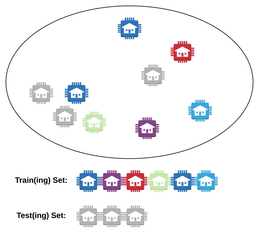
  1. Remove some houses (temporarily)
  2. Fit model on remaining (using exactly method from before)
  3. Predict heldout houses (using model of remaining houses, what values predict for removed houses)
  4. Use the predicted values, and compare to the actual observed values (use as proxy for doing the types of real predictions on data not yet collected)

This type of method will only work well if enough observations is used for fitting versus testing predictions.

Train / Test Split

Introducing a little bit of terminology.

• Train(ing) Set: the houses used to fit the model
• Test(ing) Set: the houses used as a proxy for prediction, those that are holding out

Train(ing) Error

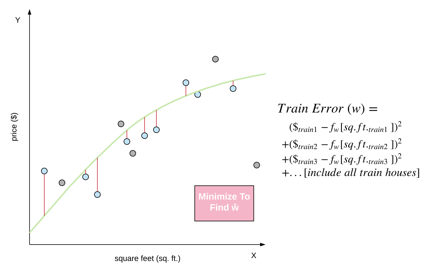
First thing to look at is something called the train(ing) error.

• Examine every house in the data set
  • Train(ing) houses are represented with blue circles
  • These are the only houses for defining the train(ing) error
  • Look at what errors are made on these house
  • This is just the residual sum of squares on the houses in the training data set (training error)

The train(ing) error looks exactly like the residual sum of squares calculation, but only including the houses that are present in the training data set.

So for any given model, such as linear fit, quadratic fit, and so on, think about estimating the model parameters as those that minimize the train(ing) error. It is equivalent to minimizing the residual sum of squares, but only looking at houses in the training data set. This is how to estimate the model parameters, $ŵ$ ($w\; (hat)$).

Test(ing) Error

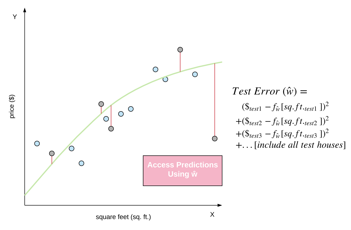
Now take these estimated model parameters to see how good they are. Need to look at the held out observations.

• Examine every house in the data set
  • Test(ing) houses are represented with gray circles
  • These houses were not used to fit the model

How well are the predicted actual house sales? When making predictions, used the value of the fit (so just the point on the line).

To assess how well are the predicted held out observations, the testing data set, look at something exactly like residual sum of squares (testing error). Take these estimated model parameter $ŵ$, and sum over the residual sum of squares over all houses that are in the testing data set.

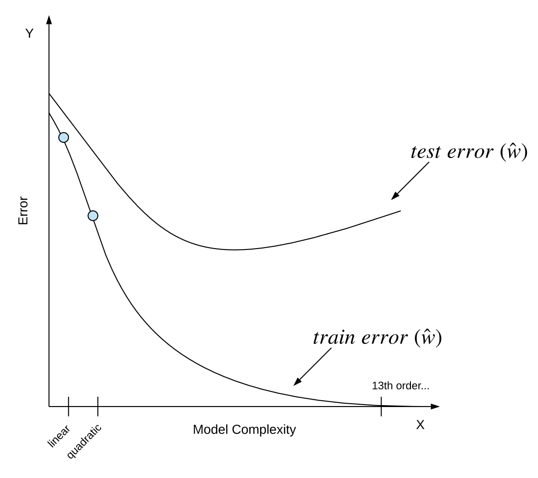
Think about how does train(ing) error and test(ing) error vary as a function of the model complexity.

Train / Test Curve

So for each model order might consider

• Train(ing) Error
  • As model order increase, the model is able to better and better fit the observation in the training data set
  • Decrease with increasing model order (flexibility of the model)
  • Residual sum of squares decrease
  • True even if some observations are held out and just look at the training data set
• Test(ing) Error
  • Expect at some point, the test(ing) error is likely to increase
  • The curve for test(ing) error maybe is going down for some period of time, but after a point, the error starts to increase again

The meaning of the variable $ŵ$ ($w\; (hat)$)

• For every model complexity, such as linear model, quadratic model, so on
• Going to optimize and find the parameters $ŵ$ for linear model, searching over all possible lines, minimize the train(ing) error
• The way to estimate the model is to minimize the error on that observation in that training data set
  • Get $ŵ$ for the linear model, compute the train(ing) error associated with that $ŵ$
  • Look at all possible quadratic fits, minimize the train(ing) error over all the quadratic fits, get $ŵ$ for the quadratic fit
  • So on…

Adding Other Features

So far assumed that the only feature relevant to the value of the house is the square feet of the house.

Prediction For House Size

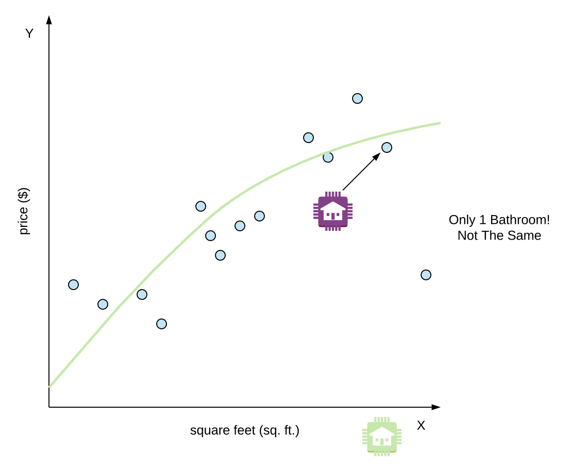
But digging into the data set a little bit more, looking at a similar house.

• The house has very similar square footage
• It is definitely making an influence on what the predictions are
• But house only have 1 bathroom, but not comparable to the current house, which has 3 bathrooms
• So the value of that house, the house sales price should not be indicative of what the current house sales price should be

Add More Feature

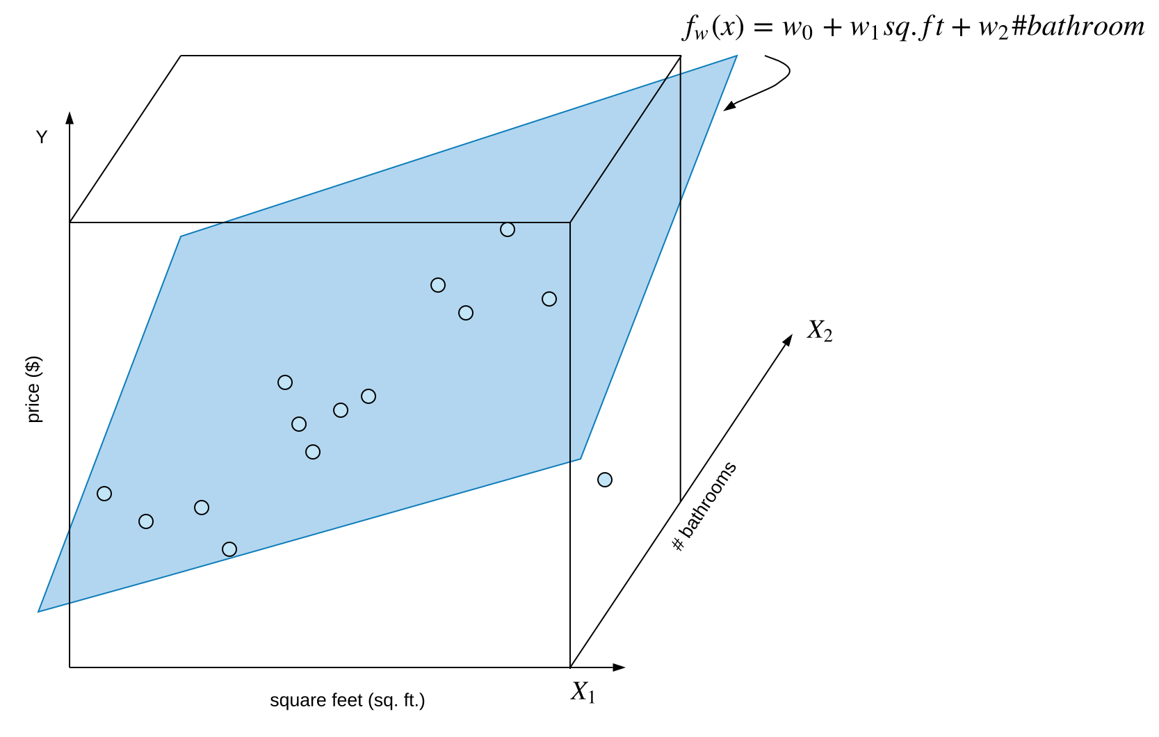
Think about adding more features.

• Instead of just looking at the relationship between square feet and price, can add number of bathroom.
  • For each one of the listings, need to go through and record how many square feet that house had, and the number of bathrooms
  • Plot each of these points in the 3D space
  • It is a hyper cube of square feet, versus bathrooms, versus price
• Instead of fitting a line to the data, thinking about just a very simple model, think about fitting a hyper plane (a slice through space)
  • Variable $w$₀ is the intercept, where the plane lives up and down on the y-axis
  • Variable $w$₁ multiply by the number of square feet
  • Variable $w$₂ multiply by the number of bathrooms

How Many Feature To Use?

A question is where to stop?

• Just want to include the number of bathrooms as additional feature
• there are a lot of things could think about including
• In addition to square feet and number of bathrooms

Possible choices:

• Number of bedrooms
• Lot size
• Year built
• …

The list goes on and on in terms of different properties (features) of the house that could be influential in assessing it’s value.

Other Regression Example

Talked quite extensively about using regression for the task of prediting house value. But the number of applications in which regression can be used are quite large.

Salary After Machine Learning Specialization

• How much will salary be? ($y\; =\; \$\$$)
• Depends on $x$
  • Performance in courses
  • Quality of capstone project
  • Number of forum response
  • So on…

Think about predicting salary, $ŷ$ ($y\; (hat)$.

• Variable $w$₀ is the intercept
• Variable $w$₁ weights on performance in the class
• Variable $w$₂ weights on quality of capstone
• Variable $w$₃ weights on participation in the forum

When estimating these model parameters, use these features (weights) for other students who have taken the course and the observations of what their salaries were, and the jobs after taking this machine learning specialization.

Stock Prediction

Think about the fact that the prediction for the price of a stock tomorrow.

• Predict the price of a stock
• Depends on
  • Recent history of stock price
  • News events
  • Related commodities

Twitter Popularity

• How many people will retweet a tweet
• Depends on
  • Number of followers
  • Number of followers of followers
  • Features of text tweeted
  • Popularity of hashtag
  • Number of past retweets
  • …

These types of models can actually be really good at predicting the eventual number of retweets of a tweet.

Smart Houses

Another very different application is maybe a smart house.

• Smart houses have many distributed sensors
• What’s the temperature at the desk (no sensor)
  • Learn (fitting) spatial function to predict temperature
• Also depends on
  • Thermostat setting
  • Blinds (open/close) or window tint
  • Vents
  • Temperature outside
  • Time of day

Summary For Regression

This module showed how regression can be used to predict house prices and also be useful in a wide range of other applications.

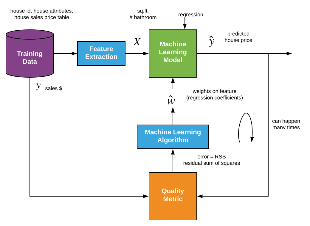
The Machine Learning Pipeline

Introduced machine learning pipeline

• Go from data
• Shoved into some machine learning method
• Use that to derive intelligence

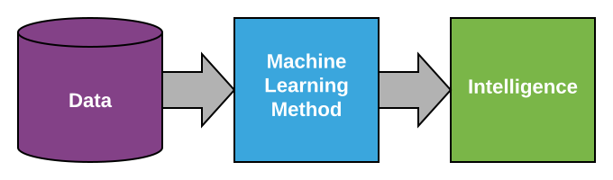
Dig into the block diagram and expand it, to see some of these machine learning tools in a little bit more detail.

• What is used to fit the data is some Training Data Set (data)
  • In the housing application for predicting the price of some house, the data collected was:
    • House ID
    • Some set of house attributes
    • House sales price
  • Had this for a whole bunch of houses in the neighborhood
  • Collected this data into some table
  • Represented the training data set
• Took that data, and shoved it through some Feature Extractor
  • In this case is a very simple feature extractor
  • Choose some subset of the house attributes
  • Variable $X$ is the set of features, represented:
    • Square feet
    • Number of bathrooms
    • Possibly using more features
• The goal was to take these features and have some type of Model that led to a prediction of the house price
  • The output, the intelligence being derived, is the predicted house price
  • Do this for every house in the training data set
    • Take its associated features
    • Shove it through this machine learning model (regression)
    • Predict the house price
• Remember that this machine learning model had some set of parameters
  • The parameters are called $ŵ$ ($w\; (hat)$)
  • These are the weights of the features
  • Weight on square feet or number of bathrooms, and so on…
  • More technically, these are called regression coefficients
  • Talked about estimating these parameters from data
  • Variable $ŵ$ is the estimate of these parameters
• Took the predicted output, so the predicted house price, and compared it to the true house price (the actual sales price recorded in the training data table)
  • Variable $y$ is the actual sales price for the houses in the training data
  • Compare to the predicted house price
• Use Quality Metric to measure how well is the prediction
  • Using the model, using $ŵ$ as the parameters of that model
• The error metric talked about was something called residual sum of squares
  • Sum up the square difference between the actual house sales price and the predicted house sales price
  • Summing over all houses in the training data set
• The Quality Metric is going to take the predicted and actual house sales observations
  • Spit out this error
  • Go into a machine learning algorithm that’s going to be used to update the weights (parameters of the model)
• The Loop where it is taking the predictions
  • Computing the error relative to the actual house sales price
  • Updating the weights of the model parameters
  • This process tends to happen in an iterative way, where the values are updated again and again

Abstract way

• Some training data set
• Some feature extraction process
• Some machine learning model
• Produce some intelligence (in this case is a prediction)
• Assess the quality of the intelligence with some quality measure
• Use that error or accuracy (depending which way to think about measuring it)
• Adjust the model parameters using some algorithm
• (Will see this type of flow for machine learning again and again)

What Can Be Done Now…

• Describe the input (features) and output (real-valued predictions) of a regression model
• Calculate a goodness-of-fit metric (e.g., RSS)
• Estimate model parameters by minimizing RSS (algorithms to come…)
• Exploit the estimated model to form predictions
• Perform a train(ing)/test(ing) split of the data
• Analyze performance of various regression models in terms of test error
• Use test error to avoid overfitting when selecting amongst candidate models
• Describe a regression model using multiple features
• Describe other applications where regression is useful

Appendix

Reference

• [PDF] Regression
• [Wikipedia] Linear Regression
• [Wikipedia] Residual Sum of Squares
• [Wikipedia] Overfitting
• [ML Wiki] Overfitting